Building a Car Model Classifier (Part 2)
This post is a continuation of the previous post.
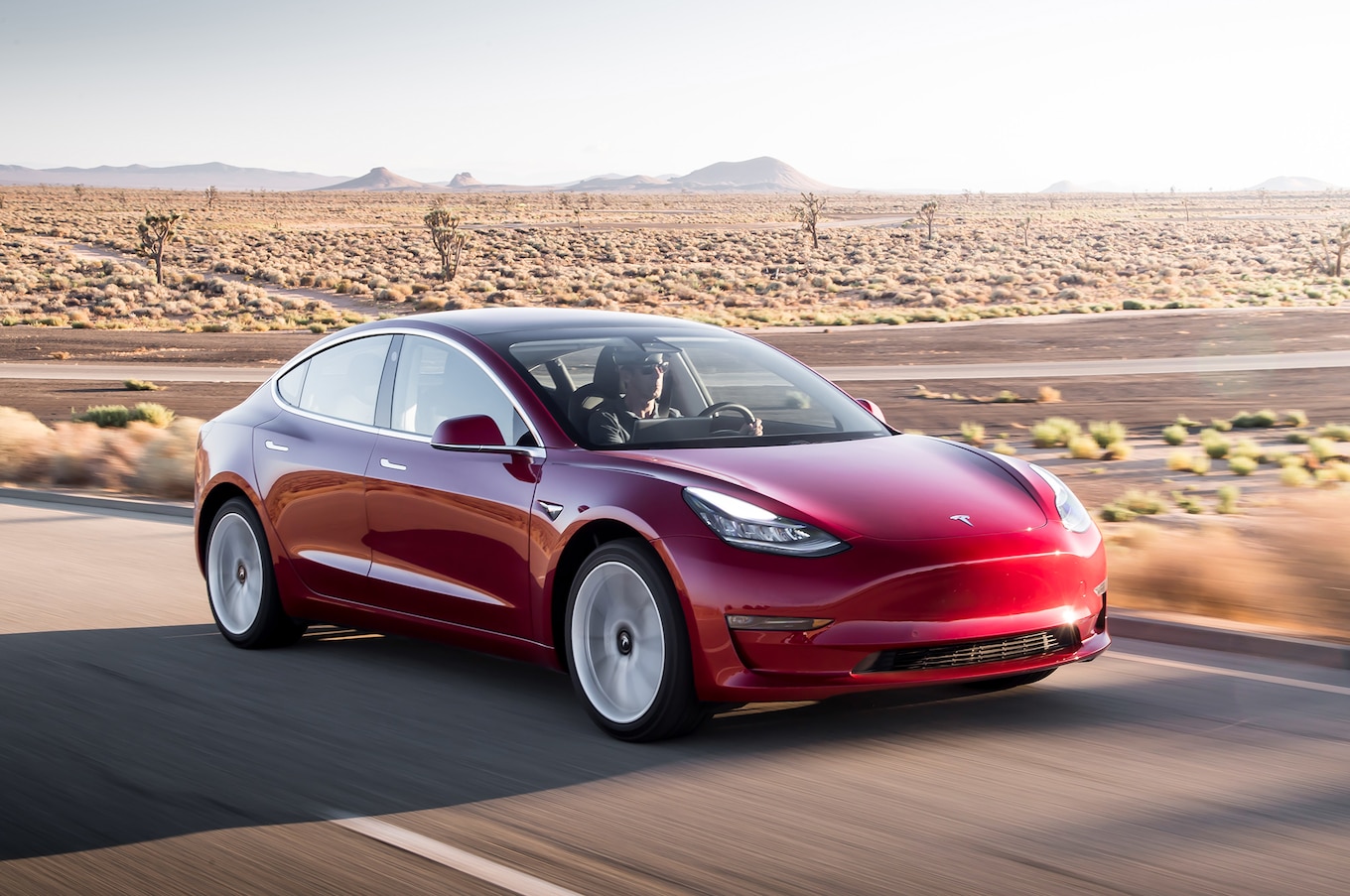
Using feature extraction and matching to nearest neighbors can only go so far with the pretrained model on VMMRdb. What if we want to generalize to newer classes of cars like the Tesla Model S, not present in the VMMRdb dataset? For that, we need to collect more data for a more updated and robust model.
Data Collection
Since there is not a collection of images of the newest car models out there, we will need to create our own dataset. And where can we find images? Google Images!
But searching, selecting N images, downloading them and organizing them by car name would take too long, so we automate it, and we do this using a web scraper.
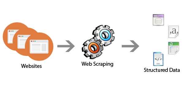
We use the NHTSA (National Highway Traffic and Safety Administration) Vehicle API, to collect a list of all the car, truck, and mpv (multi-purpose vehicle) makes and models from the year 2000 to 2018 (when this project was first started). Then we use a web scraper to create a list of links from Google Images, and finally we download them using multiprocessing because they are essentially parallel tasks.
Link to the scraper and custom scripts specifically for this project found here: scrapeCars
Data Cleaning and Preprocsesing
Data cleaning and organization is usually the most time-consuming part of a data science project, and it’s no different for this project.
Once we have all the image data, we first delete any duplicates in the same class, since we want unique samples and we can know the true size of a class, if class weighting needs to be done later.
But how can we automate duplicate removal? We can hash the images by pixel data and then store them by that hash in a database, compare the hashes and delete if they are the same. There’s a nice library that does this, found here: duplicate-images
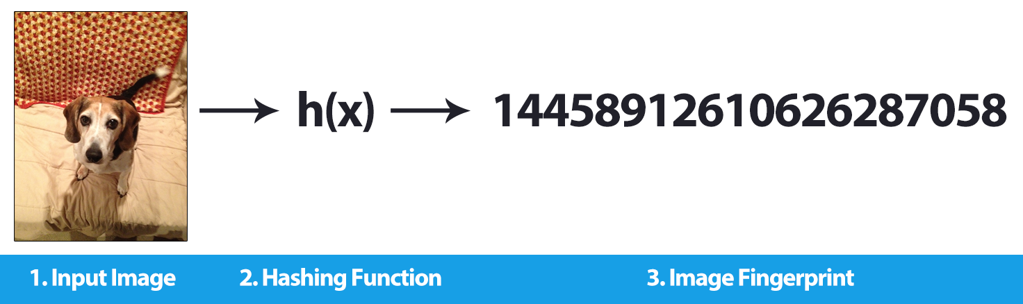
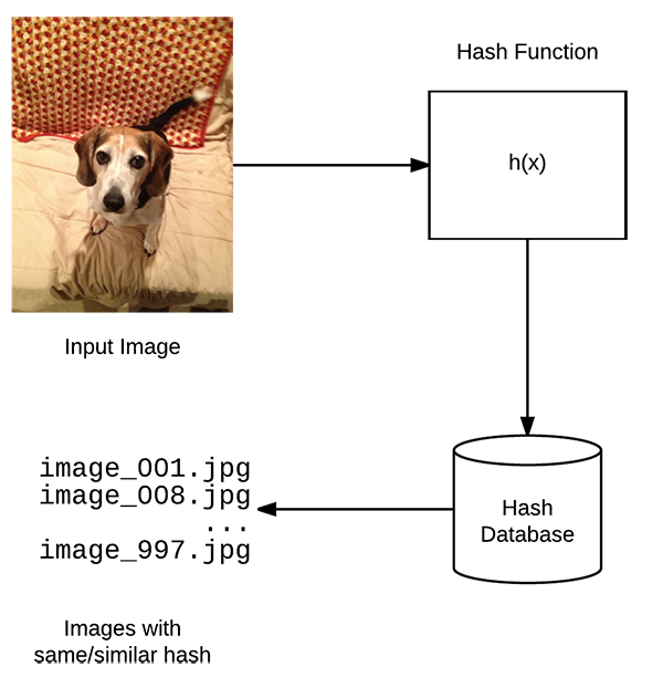
(Images from pyimagesearch)
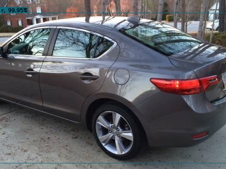
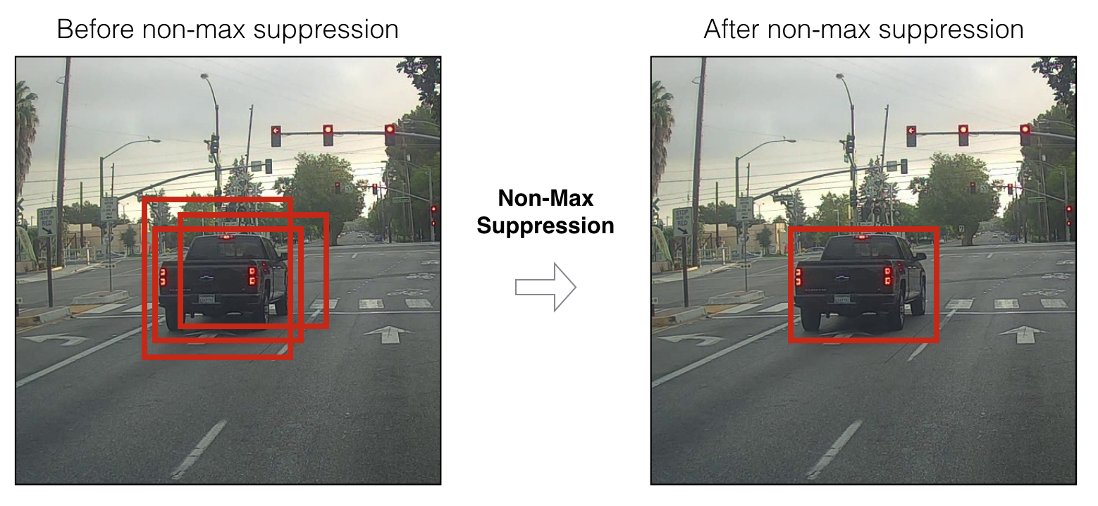
Next, our focus is classification and not detection, the difference being detection is classification + localization (finding if and where an object is present in the scene), we crop the images with only the car present, and remove most of the background. We accomplish this using YOLO v3: detect the largest bounding box of a truck or car, and crop it out. We use this library for ease of use: ImageAI
Lastly, we want to remove images that include the interior of a car: pictures steering wheels, seats, A/C, etc. I tried training a smaller model detect the differences between an image of a car and its interior to automatically remove irrelevant pictures. However, this didn’t prove to be effective because of the large variation in this type of pictures. So, I spent two to three days, going through 200k images and manually removing the bad ones.
We apply the same cropping to VMMRdb, and add it to our scraped dataset, making it effectively larger and more robust for training models since it contains good examples of certain cars and adds to smaller class sizes.
We finally have our complete dataset, and we are ready to train!
Training
Data Split
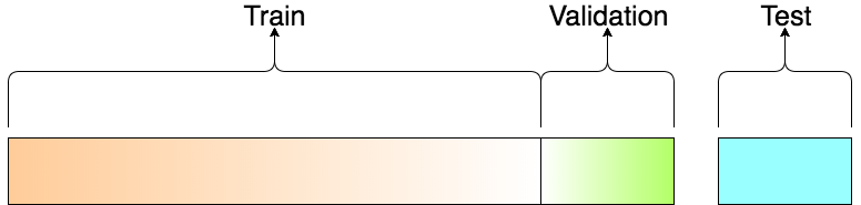
The dataset needs to be split into training, validation, and testing sets. For this we write a quick script in python to divide each class randomly into 80/10/10 for each set, respectively.
The training set is used for training the model and validation set is used to calculate the loss and accuracy after each epoch or cycle of training. Finally, the test set is untouched and unseen by the model until all the training is complete and a final loss and accuracy needs to be calculated.
Benchmarking
As a benchmark, we try out Xception, and use Tensorflow to train our model. Tensorflow 2.0 has keras built-in and it makes it easy to do a bunch of quick experiments to see if the model is training properly.
We freeze the top layers (layers closer to the input), since they are usually simple edge and shape detectors, and we unfreeze the last half of layers, allowing them to be trained. This is known as Transfer Learning, and is much faster than training a model from scratch.
We choose an image size 448x448 to preserve as much of the image as possible and apply simple image augmentations to create more varied data and thus make the model more robust to perturbations (Slight rotations, horizontal flips, color variations). Additionally, we only use the scraped dataset and not the combined dataset, since it is smaller.
We achieve a validation accuracy of 64.41% and test accuracy of 64.22%. Satisfied with this, we move on a better model and better training methods.
Better Model, Better Results
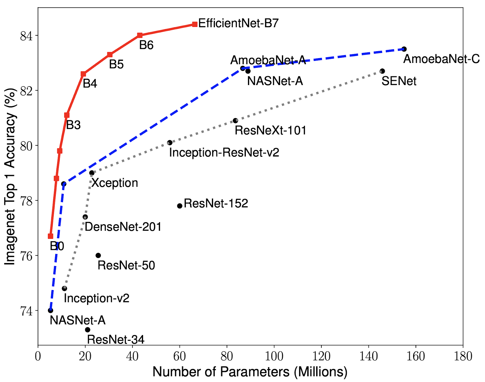
Next, we choose EfficientNet, a newer model that has ranges of models starting from B0 to B7, where the depth, width, and resolution of the models scale appropriately based on the computing resources available. They had reached the state of the art in ImageNet with a top-1 accuracy of 84.4% accuracy.
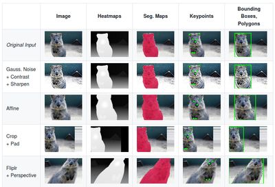
Choosing EfficientNet B0, the smallest of the set, we unfreeze the last two layers and switch to 224x224 image sizes since it takes much longer to train with 448x448 size images. We use the full dataset (VMMRdb + scraped dataset) this time and use better image augmentations as well, from this great library that has tons of augmentations: imgaug
This time we train for as long as the validation accuracy does not improve for 8 epochs. We use Adam with a starting learning rate of 1e-4, this was discovered with trial and error. After about 18 epochs of training, we stop and get a final training accuracy of 86.66% and validation accuracy of 80.18%.
On the test set, we get an accuracy of 80.1%! Almost a 16% increase from using the combined dataset, a better model, and better image augmentations.
This is part 2 of my progress towards this problem, stay tuned for my next and last post on this topic, where I build a final pipeline for the classification.